MAG Generation

MAG generation
- Generation of metagenome assembled genomes (MAGs) from assemblies
- Assessment of quality
- Taxonomic assignment
- Visualisation of taxonomy tree
Prerequisites
For this tutorial, you will need to start the docker container by running the following command in the terminal:
chmod a+rwx -R /home/training/course_dir/work_dir/Day_2/binning
docker pull quay.io/microbiome-informatics/mags-practical-2025:latest
docker run --rm --user 1001:1001 -it -v /home/training/course_dir/work_dir/Day_2/binning:/opt/data quay.io/microbiome-informatics/mags-practical-2025
Generating metagenome assembled genomes
Learning Objectives - in the following exercises, you will learn how to bin an assembly, assess the quality of this assembly with СheckM and CheckM2, define GTDB and NCBI taxonomies and then visualize a placement of these genomes within a reference tree.
As with the assembly process, there are many software tools available for binning metagenome assemblies. Examples include, but are not limited to:
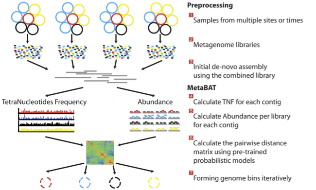
There is no clear winner between these tools, so it is best to experiment and compare a few different ones to determine which works best for your dataset. For this exercise, we will be using MetaBAT (specifically, MetaBAT2). The way in which MetaBAT bins contigs together is summarized in Figure 1.
Preparing to run MetaBAT
Prior to running MetaBAT, we need to generate coverage statistics by mapping reads to the contigs. To do this, we can use bwa and then the samtools software to reformat the output. This can take some time, so we have run it in advance.
Let’s browse the files that we have prepared:
cd /opt/data/assemblies/
ls
You should find the following files in this directory:
contigs.fasta: a file containing the primary metagenome assembly produced by metaSPAdes (contigs that haven’t been binned)input.fastq.sam.bam: a pre-generated file that contains reads mapped back to contigs
If you are very interested to generate the input.fastq.sam.bam file yourself, you can run the following commands (but better do it in the end of practical if you have time left):
# NOTE: you will not be able to run subsequent steps until this workflow is completed because you need
# the input.fastq.sam.bam file to calculate contig depth in the next step. In the interest of time, we
# suggest that if you would like to try the commands, you run them after you complete the practical.

# If you would like to practice generating the bam file, back up the input.fastq.sam.bam file that we
# provided first, as these steps will take a while:

cd /opt/data/assemblies/
mv input.fastq.sam.bam input.fastq.sam.bam.bak

# index the contigs file that was produced by metaSPAdes:
bwa index contigs.fasta

# fetch the reads from ENA
wget ftp://ftp.sra.ebi.ac.uk/vol1/fastq/ERR011/ERR011322/ERR011322_1.fastq.gz
wget ftp://ftp.sra.ebi.ac.uk/vol1/fastq/ERR011/ERR011322/ERR011322_2.fastq.gz

# map the original reads to the contigs:
bwa mem contigs.fasta ERR011322_1.fastq.gz ERR011322_2.fastq.gz > input.fastq.sam

# reformat the file with samtools:
samtools view -Sbu input.fastq.sam > junk
samtools sort junk -o input.fastq.sam.bam
Running MetaBAT
cd /opt/data/assemblies/
mkdir contigs.fasta.metabat-bins2000
In this case, the directory might already be part of your VM, so do not worry if you get an error saying the directory already exists. You can move on to the next step.
Run the following command to produce a contigs.fasta.depth.txt file, summarizing the output depth for use with MetaBAT:
jgi_summarize_bam_contig_depths --outputDepth contigs.fasta.depth.txt input.fastq.sam.bamNow let’s put together the metaBAT2 command. To see the available options, run:
metabat2 -hHere is what we are trying to do:
we want to bin the assembly file called
contigs.fastathe resulting bins should be saved into the
contigs.fasta.metabat-bins2000folderwe want the bin file names to start with the prefix
binwe want to use the contig depth file we just generated (
contigs.fasta.depth.txt)the minimum contig length should be 2000
Take a moment to put your command together but please check the answer below before running it to make sure everything is correct.
See the answer
metabat2 --inFile contigs.fasta --outFile contigs.fasta.metabat-bins2000/bin --abdFile contigs.fasta.depth.txt --minContig 2000Once the binning process is complete, each bin will be grouped into a multi-fasta file with a name structure of **bin.[0-9]*.fa**.
Inspect the output of the binning process.
ls contigs.fasta.metabat-bins2000/bin*How many bins did the process produce?
How many sequences are in each bin?
Quality assessment
Obviously, not all bins will have the same level of accuracy since some might represent a very small fraction of a potential species present in your dataset. To further assess the quality of the bins, we will use CheckM.
Running CheckM v1.2.4
CheckM has its own reference database of single-copy marker genes. Essentially, based on the proportion of these markers detected in the bin, the number of copies of each, and how different they are, it will determine the level of completeness, contamination, and strain heterogeneity of the predicted genome.
Before we start, we need to configure CheckM.
cd /opt/data
mkdir /opt/data/checkm_data
tar -xf checkm_data.tar.gz -C /opt/data/checkm_data
checkm data setRoot /opt/data/checkm_data
This program has some handy tools not only for quality control but also for taxonomic classification, assessing coverage, building a phylogenetic tree, etc. The most relevant ones for this exercise are wrapped into the lineage_wf workflow.
This command uses a lot of memory. Do not run anything else while executing it.
cd /opt/data/assemblies
checkm lineage_wf -x fa contigs.fasta.metabat-bins2000 checkm_output --tab_table -f MAGs_checkm.tab --reduced_tree -t 4
Due to memory constraints (< 40 GB), we have added the option --reduced_tree to build the phylogeny with a reduced number of reference genomes.
Once the lineage_wf analysis is done, the reference tree can be found in checkm_output/storage/tree/concatenated.tre.
Additionally, you will have the taxonomic assignment and quality assessment of each bin in the file MAGs_checkm.tab with the corresponding level of completeness, contamination, and strain heterogeneity (Fig. 2). A quick way to infer the overall quality of the bin is to calculate the level of **(completeness - 5*contamination). You should be aiming for an overall score of at least 70-80%**. We usually use 50% as the lowest acceptable cut-off (QS50)
You can inspect the CheckM output with:
cat MAGs_checkm.tabComparing CheckM and CheckM2
Today researchers also use CheckM2, an improved method of predicting genome quality that uses machine learning. The execution of CheckM2 takes more time than CheckM. We have pre-generated the tab-delimited quality table with Checkm2 v1.1.0. It is available on our FTP.
FYI command that was used to generate CheckM2 output:
checkm2 predict -i contigs.fasta.metabat-bins2000 -o checkm2_result --database_path CheckM2_database/uniref100.KO.1.dmnd -x fa --force -t 16Download the CheckM2 result table that we have pre-generated:
# create a folder for the CheckM2 result
cd /opt/data/assemblies
mkdir checkm2
cd checkm2
# download CheckM2 TSV result
wget https://ftp.ebi.ac.uk/pub/databases/metagenomics/mgnify_courses/metagenomics_2025/mags/checkm2_quality_report.tsv
We can compare CheckM and CheckM2 results using a scatter plot. We will plot completeness on the x-axis and contamination on the y-axis. We have created a simple python script to plot CheckM and CheckM2 results separately. Input table should be in the CSV format and it should contain 3 columns: bin name, completeness, and contamination. Required file header: “bin,completeness,contamination”
Modify the CheckM results table and generate a plot:
# modify MAGs_checkm.tab
# add header
echo "bin,completeness,contamination" > checkm1_quality_report.csv
# take the file without the header; leave only columns 1, 12 and 13; replace tabs with commas
tail -n+2 MAGs_checkm.tab | cut -f1,12,13 | tr '\t' ',' >> checkm1_quality_report.csv

# plot
completeness_vs_contamination.py -i checkm1_quality_report.csv -o checkm1Now do the same for CheckM2. Modify the table and make a plot:
# create CSV
# add a header
echo "bin,completeness,contamination" > checkm2_quality_report.csv
# take the file without the header, leave only the first 3 columns, replace tabs with commas
tail -n+2 checkm2_quality_report.tsv | cut -f1-3  | tr '\t' ',' >> checkm2_quality_report.csv

# plot
completeness_vs_contamination.py -i checkm2_quality_report.csv -o checkm2
You should now have files checkm1.png and checkm2.png to compare the quality predictions between the two tools. To open the png files, use the file browser (grey folder icon in the left-hand side menu) and navigate to /home/training/course_dir/work_dir/Day_2/binning/assemblies
Did CheckM and CheckM2 produce similar results? What can you say about the quality of the bins? How many bins pass QS50?
Quality filtering
Usually bins with bad quality are not included into further analysis. In MGnify we use criteria: 50 <= completeness <= 100 and 0 <= contamination <= 5 or more strict rule QS50: completeness - 5 x contamination >= 50.
In our example, ideally we should exclude bin.1, bin.2 and bin.9 but we left those in the practical in order to see how different tools manage bad quality bins.
Dereplication
Another mandatory step that should be done in MAGs generation is dereplication of bins. This process includes identifying and removing redundant MAGs from a dataset by clustering bins based on their similarity, typically using Average Nucleotide Identity (ANI), and then selecting the highest-quality representative from each cluster. The most popular tool is dRep but, unfortunately, we do not have enough time to launch it during that practical. You can browse documentation of dRep if you are interested.
Taxonomy assignment
GTDB-Tk taxonomy
A commonly used tool to determine genome taxonomy is GTDB-Tk. The taxonomy is built using phylogenomics (based on conserved single-copy marker genes across >300,000 bacterial/archaeal genomes) and regularly updated. Due to the long time it takes to run it, we have already launched GTDB-Tk v2.4.1 with DB release v226 on all bins and saved the results to the FTP. Let’s take a look at the assigned taxonomy.
FYI command that was used to generate GTDB-Tk output:
gtdbtk classify_wf --cpus 16 --pplacer_cpus 8 --genome_dir contigs.fasta.metabat-bins2000 --extension fa --skip_ani_screen --out_dir gtdbtk_resultsDownload and check taxonomy file.
cd /opt/data/assemblies

# download the table
wget https://ftp.ebi.ac.uk/pub/databases/metagenomics/mgnify_courses/metagenomics_2025/mags/taxonomy/bins_v226_gtdbtk.bac120.summary.tsv

# the first two columns of the table contain the bin name and the assigned taxonomy - take a look:
cut -f1,2 bins_v226_gtdbtk.bac120.summary.tsvHow many bins were classified to the species level?
Make a guess why some bins were not assigned to any pylum?
GTDB vs NCBI taxonomy
Another widely used taxonomy is from NCBI but, unfortunately, GTDB and NCBI taxonomies are differ in their goals, methodology, and naming rules. NCBI taxonomy contains all organisms (bacteria, archaea, eukaryotes, viruses) but GTDB has only bacteria and archaea. Submission to NCBI is integrated with GenBank, RefSeq, SRA, and most bioinformatics pipelines. Taxonomy is built on historical taxonomic assignments (literature, culture collections) but it might be inconsistent (different ranks may not reflect phylogeny). Many bioinformatics tools and pipelines require NCBI taxID assigned for your data. It is possible to assign it with CAT or convert existing GTDB taxonomy into NCBI using script gtdb_to_ncbi_majority_vote.py provided by GTDB-Tk developers.
As we already have GTDB taxonomy lets convert it into NCBI. Converter input is full gtdb-tk output folder and metadata files for bacteria and archaea.
cd /opt/data/assemblies

# download the archive with gtdb-tk result
wget https://ftp.ebi.ac.uk/pub/databases/metagenomics/mgnify_courses/metagenomics_2025/mags/taxonomy/gtdbtk_results.tar.gz

# uncompress archive
tar -xzf gtdbtk_results.tar.gz

# download metadata for archaea
wget https://ftp.ebi.ac.uk/pub/databases/metagenomics/mgnify_courses/metagenomics_2025/mags/taxonomy/ar53_metadata_r226.tsv

# download metadata for bacteria
wget https://ftp.ebi.ac.uk/pub/databases/metagenomics/mgnify_courses/metagenomics_2025/mags/taxonomy/bac120_metadata_r226.tsv

# run a converter
gtdb_to_ncbi_majority_vote.py --gtdbtk_output_dir gtdbtk_results --output_file gtdb_ncbi_taxonomy.txt --ar53_metadata_file ar53_metadata_r226.tsv --bac120_metadata_file bac120_metadata_r226.tsvDo you find any differences in assigned taxonomies?
Compare those lineages with Checkm results. What do you see?
Defining Taxonomy Identifier (TaxID)
A taxonomy identifier (often called taxid) is a numeric identifier assigned to a taxon (species, genus, etc.) in a taxonomy database. It’s a stable way to refer to a taxon without relying on names, which can change. The simplest way to search for it is using Taxonomy Browser. You can also use ENA Text search.
Can you determine TaxID for all bins (if the species-level TaxId is not known, a TaxId for a higher taxonomic level can be used)? Try to search for GTDB lineage. What can you see in taxonomy for bin.5?
Visualizing the phylogenetic tree
Now you can visualise your classified bins on a small bacterial phylogenetic tree with iTOL. A quick and user-friendly way to do this is to use the web-based interactive Tree of Life iTOL. To use iTOL you will need a user account. For the purpose of this tutorial we have already created one for you with an example tree. iTOL only takes in newick formatted trees.
That tree was generated with tool FastTree from a subset of sequences from multiple sequence alignment generated by GTDB-Tk tool. Alignment can be found in GTDB-Tk result folder gtdbtk_results/align/gtdbtk.bac120.msa.fasta.
FYI commands that were used to generate the tree:
# subsequence alignment file gtdbtk_results/align/gtdbtk.bac120.msa.fasta with seqkit tool to pick clades with bins
# then build a tree
FastTree -out small_bac_tree.nwk gtdbtk_results/align/gtdbtk.bac120.msa.chosen.fasta- Pre-download tree files from FTP:
- tree: https://ftp.ebi.ac.uk/pub/databases/metagenomics/mgnify_courses/metagenomics_2025/mags/taxonomy/small_bac_tree.nwk
- legend by phylum: https://ftp.ebi.ac.uk/pub/databases/metagenomics/mgnify_courses/metagenomics_2025/mags/taxonomy/small_bac_tree.legend.txt
- layers by phylum: https://ftp.ebi.ac.uk/pub/databases/metagenomics/mgnify_courses/metagenomics_2025/mags/taxonomy/small_bac_tree.layer.txt
Rename files with prefix: your_name_training25.
Go to the iTOL website (open the link in a new window).
Login is as follows:
User: EBI_training
Password: EBI_training
After you login, just click on My Trees in the toolbar at the top
From there select Tree upload and upload tree file with .nwk extension.
Once uploaded, click the tree name to visualize the plot
To colour the clades and the outside circle according to the phylum of each strain, drag and drop the files .legend.txt and .layer.txt
Now you can play a bit with tree using Control panel on the left. For example, try to visualise Unrooted tree (Control panel -> Basic -> Mode -> Unrooted).
As we built the tree from GTDB-Tk result we can easily assign taxonomy to tree nodes in iTOL. Go to: Control Panel -> Advanced -> Other functions -> Auto assign taxonomy -> GTDB.
How to find our bins on the tree? For example, try to find bin.7.
Hint: Use a magnifier with Aa sign on the left of the iTOL window and search for species name.
What else can I do with MAGs?
Once MAGs are recovered, annotation is a critical step in turning raw sequence data into biological knowledge. We have already done Taxonomic annotation.
It is also useful to have:
Structural annotation – predicting genes, coding sequences (CDS), rRNAs, tRNAs, and other genomic features.
Functional annotation – assigning putative functions to predicted genes using homology searches against protein/domain databases (e.g., KEGG, Pfam, eggNOG, InterPro).
There are many pipelines available for MAGs annotation. MGnify team wildly uses pipeline mettannotator or you can also check nf-core mag pipeline.